Box Spread Solution

Task 1

import numpy as np
import matplotlib.pyplot as plt
import statsmodels.api as sm
import pandas as pd

df = pd.read_csv("data/spx_option_data.csv")
# Filter the data for options with 352 days to maturity
df_352 = df[df['maturity'] == 352].copy()

# Compute the put-call differential
df_352['put_call_diff'] = df_352['put_price'] - df_352['call_price']

# Perform a linear regression of put-call differential against strike price
X = df_352['strike']
y = df_352['put_call_diff']
X = sm.add_constant(X)  # Add constant for intercept

model = sm.OLS(y, X).fit()
slope = model.params[1]

# Compute implied box rate R_T
T_days = 352
R_T = 1 / slope

# Plot put-call differential against strike price
plt.figure(figsize=(8, 5))
plt.scatter(df_352['strike'], df_352['put_call_diff'], label="Put-Call Differential", alpha=0.7)
plt.plot(df_352['strike'], model.predict(X), color='red', label="Regression Line")
plt.xlabel("Strike Price")
plt.ylabel("Put-Call Differential")
plt.title("Put-Call Differential vs. Strike Price")
plt.legend()
plt.grid(True)
plt.show()

# Calculate cost of synthetic long at K=4000 and synthetic short at K=6000
K1, K2 = 4000, 6000
box_spread_cost = df_352.loc[df_352['strike'] == K2, 'put_call_diff'].values[0] - \
                   df_352.loc[df_352['strike'] == K1, 'put_call_diff'].values[0]

# Risk-free payoff at T
box_spread_payoff = K2 - K1

# Display results
print(f"Implied Box Rate (R_T): {R_T}")
print(f"Upfront Cost for Box Spread: {box_spread_cost}")
print(f"Risk-Free Payoff in 352 Days: {box_spread_payoff}")

Implied Box Rate (R_T): 1.0102565338916818
Upfront Cost for Box Spread: 1979.65
Risk-Free Payoff in 352 Days: 2000

Task 2

# Compute the left-hand side (LHS) of put-call parity: P - C
lhs = df_352['put_call_diff']

# Compute the right-hand side (RHS) of put-call parity: K * e^(-rT) - S0
discount_factor = 1 / R_T  # e^(-rT)
rhs = df_352['strike'] * discount_factor - df_352['spx']

# Plot LHS against RHS with a 45-degree line
plt.figure(figsize=(7, 7))
plt.scatter(rhs, lhs, label="Put-Call Parity", alpha=0.7)
plt.plot([min(lhs), max(lhs)], [min(lhs), max(lhs)], color='red', linestyle="--", label="45-degree Line")
plt.xlabel("Right-Hand Side (K * e^(-rT) - S0)")
plt.ylabel("Left-Hand Side (P - C)")
plt.title("Checking Put-Call Parity")
plt.legend()
plt.grid(True)
plt.show()

Task 3

import pandas as pd
import numpy as np
import matplotlib.pyplot as plt
import statsmodels.api as sm

# Load datasets
option_file_path = "data/spx_option_data.csv"  # Update with your file path
treasury_file_path = "data/treasury_yield.csv"

df_options = pd.read_csv(option_file_path)
df_treasury = pd.read_csv(treasury_file_path)

# Compute box rates for each available maturity in the option dataset
maturity_groups = df_options.groupby('maturity')

box_rates = []

for maturity, group in maturity_groups:
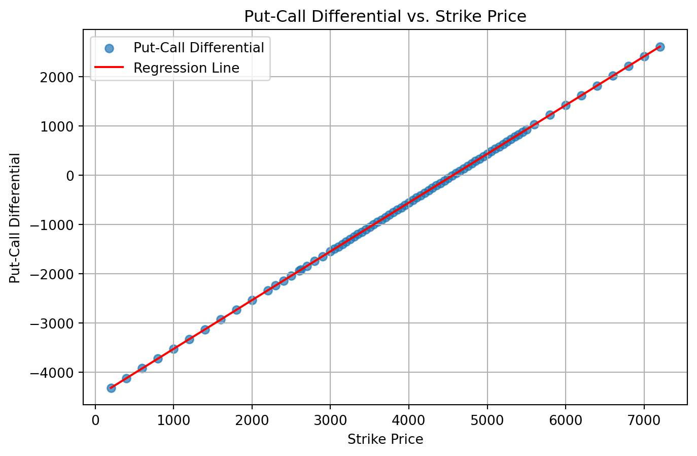
    X = group['strike']
    y = group['put_price'] - group['call_price']
    X = sm.add_constant(X)  # Add intercept

    model = sm.OLS(y, X).fit()
    slope = model.params[1]

    # Compute box rate and correctly annualize it: (R_T)^(360/T) - 1
    R_T = 1 / slope
    annualized_R_T = (R_T ** (360 / maturity)) - 1
    
    box_rates.append({'maturity_days': maturity, 'box_rate': annualized_R_T * 100})  # Convert to percentage

# Convert to DataFrame
df_box_rates = pd.DataFrame(box_rates)
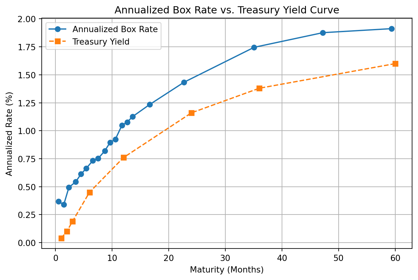
df_box_rates['maturity_months'] = df_box_rates['maturity_days'] / 30

# Plot the annualized box rate against maturity in months
plt.figure(figsize=(8, 5))
plt.plot(df_box_rates['maturity_months'], df_box_rates['box_rate'], marker='o', linestyle='-', label="Annualized Box Rate")

# Overlay the Treasury yield curve
plt.plot(df_treasury['months'], df_treasury['tbill_rate'], marker='s', linestyle='--', label="Treasury Yield")

plt.xlabel("Maturity (Months)")
plt.ylabel("Annualized Rate (%)")
plt.title("Annualized Box Rate vs. Treasury Yield Curve")
plt.legend()
plt.grid(True)
plt.show()