Box Spread
This project will guide you in creating a box spread using the put-call parity. We show that by combining different positions in highly nonlinear and risky options, we can recreate a risk-free payoff. This risk-free payoff is typically referred to as the “box spread”.
For further reading on box spreads, please refer to this article from the NY Fed.
Recap on the Put-Call Parity and the Box Spread
Recall that the put-call parity is given by:
\[ C - P = S_0 - K e^{-rT} \]
where \(C\) is the price of a call option, \(P\) is the price of a put option, \(S_0\) is the current price of the underlying asset, \(K\) is the strike price, and \(r\) is the risk-free rate.
The put call parity says that a long call and a short put with the same strike price \(K\) and at the same expiration date is equivalent to borrowing \(K\) to buy the underlying asset. In other words, it creates a synthetic long position.
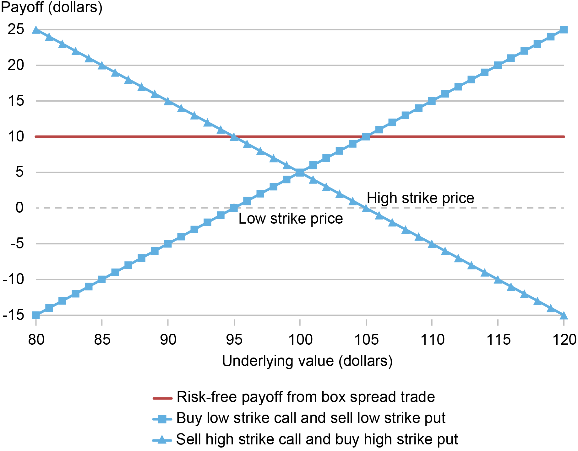
By taking a synthetic long position at the low strike price and a synthetic short position at the high strike price, we create a risk-free payoff as follows:

Mathematically, we have:
\[ \left.\begin{array}{c} C^{L}-P^{L}=S_{0}-K^{L}e^{-rT}\\ -(C^{H}-P^{H})=-(S_{0}-K^{H}e^{-rT}) \end{array}\right\} \implies\underset{\text{Initial Investment}}{\underbrace{C^{L}-P^{L}-(C^{H}-P^{H})}}=\underset{\text{Riskfree Payoff}}{\underbrace{(K^{H}-K^{L})e^{-rT}}} \]
where \(C_L\) is the price of a call option with the low strike price, \(P_H\) is the price of a put option with the high strike price, \(C_H\) is the price of a call option with the high strike price, and \(P_L\) is the price of a put option with the low strike price.
If we have multiple strike prices at the same expiration date \(T\), the equation above implies that the put-call price differentials should fall on a straight line as a function of the strike price \(K\). That is:
\[P_T(K) - C_T(K) = a_T + b_T K \]
where \(b_T \equiv e^{-rT}\) is the discount rate. This suggests that we can estimate the discount rate at each horizon \(T\) by running a cross-sectional regression of the put-call price differential on the strike price \(K\).
Task 1: Plot the Put-Call Differential Against the Strike Price
Steps:
- Download and load this dataset. It is a sample of SPX option prices from the CBOE on 02/02/2022.
- Use only the subsample with 352 days to maturity (
maturity == 352). - Compute the put-call differential, defined as the put price minus the call price, and plot it against the strike price.
- Report the implied box rate \(R_T\) from the slope of the regression line. Notice that the slope is \(b_T = e^{-rT} = \frac{1}{R_T}\), and in this case, \(T=352\) days.
- Given the information from the figure, if you take a synthetic long at \(K=4000\) and a synthetic short at \(K=6000\) using the given options, how much would you pay upfront for the box spread? What would be the payoff in 352 days? Convince yourself that no matter what the level of the SPX is in 352 days, the payoff is risk-free.
Hint: The figure would look like this:
Task 2: Check Put-Call Parity
Using the \(R_T\) computed from above, check that the put-call parity holds for the subsample with 352 days to maturity.
Recall that the put-call parity is given by (flip the signs to be consistent with the figure above):
\[ P - C = K e^{-rT} - S_0 \]
We can check this by plotting the left-hand side against the right-hand side. To compute the right-hand side, use the column spx as the current price of the underlying asset, i.e., the SPX index level, and use the box rate computed in the previous task for \(e^{-rT}\).
- Plot the left-hand side against the right-hand side in a scatter plot.
- Add a 45-degree line to the plot to see if the points fall on the line.
Hint: The scatter plot will be very close to the 45-degree line, but with a very slight difference. This suggests the existence of a very small arbitrage opportunity in the real world.
Task 3: Compare the Box Rate Yield Curve with the Treasury Yield
The yield curve visualizes the relationship between the risk-free rate and maturity. In the tasks above, we only used one maturity at \(T=352\). Now, compute box rates at different maturities and plot them against the Treasury yield.
- For a subsample of each maturity available in the dataset, run the regression of the put-call differential on the strike price and compute the corresponding box rate as in Task 1. Notice that the box rate implied from the regression is for the maturity \(T\). To compare it across the yield curve, annualize it by multiplying it by \(360/T\).
- Plot the annualized box rate against the maturities in months.
- Load the Treasury yield data from this file. It is the yield curve on Treasury securities with different maturities on 02/02/2022, retrieved from Treasury.gov. Overlay the Treasury yield on the box rate plot.
Hint: You should get a figure with the box rates slightly higher than the Treasury yields across all maturities, indicating that Treasury securities are relatively overpriced compared to the prevailing interest rate in the derivative market and hence offer lower returns. The difference is typically referred to as the “convenience yield” of the Treasury securities.